
The Concept of Time Borrowing and Useful Skew
- saumil vora

- Nov 1, 2020
- 4 min read
1. Time Borrowing
In the last blog, we discussed various techniques to fix the timing violations (click here to read). In the setup timing analysis section, the latch based approach was discussed in one of the points. We will discuss the latch based approach to fix the setup timing in detail in this blog. Latch based technique is also known as the time borrowing technique or the cycle stealing technique.
To understand the need for a latch based approach, let us consider a flop to flop path as shown in figure 1.
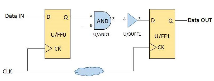
Here, let us assume that the setup timing is unable to meet for this path. Even after trying all possible optimizations, the setup timing is still violating. So now options available with us are to change the frequency or we can use a latch at the place if capture flop (U/FF1). Unlike flip-flop, a latch is transparent for the entire level thus offers extra time to capture the data. This reduces the available time for the next path. This concept is known as time borrowing as time is borrowed from the next cycle. Let us understand this with the help of an example.
Example: Positive Launch Flop and Positive Latch


If data arrives at U/L1 at point A (as shown in the waveform), then the operation is the same as in the case of flop to flop path. In our example, this is not the case. Data is arriving at point B (60ps). As a positive latch is transparent for the entire positive level, data will be captured by the latch and processed further. In doing so, we have 10ps less in the next cycle. Instead of a 50ps time window from point A to C (refer waveform), we have a 40ps time window for the next cycle from point B to C. Eventually we are able to meet the setup time in path U/FF0 to U/L1 but at the cost of setup margin from the subsequent path. Here if data at U/L1 arrives after its positive level i.e. at the falling edge of U/L1 then setup will violate for path U/FF0 to U/L1. One more thing to take care of before using the latch at capture position is that we must have enough hold margin. This is because the latch will remain transparent for the entire positive level and meanwhile new data should not reach the latch input otherwise the path will enter into the metastable state.
From this example, it can be concluded that we can use the latch based approach only if we have enough setup margin in the subsequent paths and enough hold margin in the current path.
2. Useful Skew
Like time borrowing, useful skew is also a technique to improve timing violations. In useful skew, we play with the clock path instead of using a latch. To meet setup time with the useful skew technique, we have to delay the clock at capture clock path. The reason for doing so is that setup time violates when the clock reaches earlier than the data at the capture flop. Hence, the idea is to delay the capture clock. Let us understand it with the help of a figure.

As it can be seen in figure 3, two inverters U/CKINV1 and U/CKINV2 are added near the clock pin of the capture clock so that it cannot affect the remaining clock path. With this, we have delayed the capture clock by the propagation delay of the two inverters. Hence data will get extra time to reach the capture flop.
Before adding inverters, one should check for the hold margin in the same path and setup the margin in the subsequent path. If anyone of them is not available then there is no meaning in implementing the useful skew technique. Useful skew can also be used to fix hold timing by increasing the delay of the launch clock path. In this case, also cells are added near to the launch clock pin.
3. Difference Between Time Borrowing and Useful Skew Techniques
In the time borrowing technique, a latch (at the place of a flop) is used to meet the timing requirements while in the useful skew technique we change the delay of the clock path.
In the time borrowing technique, the time is borrowed from the subsequent cycle reducing the effective clock cycle for the succeeding path. Whereas in useful skew technique clock cycle itself is delayed but not borrowed from the subsequent path. All the paths get the complete cycle.
The use of latches makes the timing analysis difficult. STA tool takes more time to perform analysis if more number of latches are used. This is a major drawback of using a latch to meet timing requirements. This problem does not occur in the case of useful skew.
The main motive for this blog is to understand the concepts of time borrowing, the useful skew, and the difference between both the techniques. For any queries or feedback please mention in the comment section below.
To read other blogs on physical design concepts click on the below links.


Comments